Training Your Own Voice Font Using Flowtron

Recent conversational AI research has demonstrated automatically generating high quality, human-like audio from text. For example, you can use Tacotron 2 and WaveGlow to convert text into high quality, natural-sounding speech in real time. You can also use FastPitch to generate mel spectrograms in parallel, achieving good speedup compared to Tacotron 2.

However, current text-to-speech models do not give you enough control over how the generated speech sounds, disregarding the acoustic properties of the voice. Such non-textual information, conveying the meaning and human expressiveness, is difficult to express because they are unlabeled. For example, it is unclear how to label audio samples with the same text but different emphasis or emotion.

Without labels available, works like Tacotron-GST and Tacotron GM-VAE have proposed using learned latent embeddings to regard the non-textual information. These models are hard to train, require guessing the dimensionality of the latent embedding, provide limited control over variability, and do not allow for manipulation of the latent space over time.

Flowtron is an easy to train, autoregressive, flow-based, generative network for speech synthesis, maximizing control over speech variation and style transfer. Flowtron allows you to transfer characteristics from a style sample or speaker to a target speaker. You can listen to many interesting audio samples and variations generated with Flowtron on the NVIDIA Applied Deep Learning Research (ADLR) group page. The audio quality of samples generated with Flowtron matches that of state-of-the-art models in terms of mean opinion scores (MOS). Using Flowtron, you can either train the model from scratch if you have a large dataset, or fine-tune the pretrained models if you have a small dataset.

This post, intended for developers with professional understanding of deep learning, helps you produce an expressive text-to-speech model for customization.

What is Flowtron?

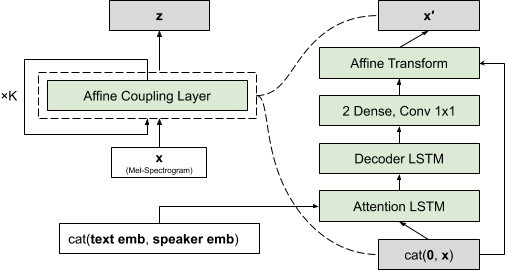
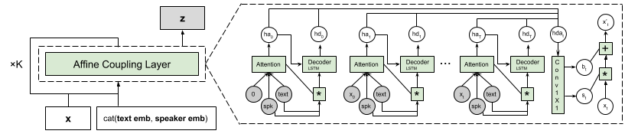
As an autoregressive model, Flowtron generates a sequence of mel-spectrogram frames by producing each mel-spectrogram frame based on the previous mel-spectrogram frames. Flowtron is composed of a text encoder that generates text embeddings, and a decoder with a stack of neural networks (affine coupling layers) that transform random noise into mel spectrograms, as shown in Figure 1.

The text encoder modifies the text encoder of Tacotron 2 by replacing batch-norm with instance-norm, and the decoder removes the pre-net and post-net layers from Tacotron previously thought to be essential. For more information, see Flowtron: an Autoregressive Flow-based Generative Network for Text-to-Speech Synthesis.

The invertible affine coupling layers produce the scaling and bias terms for the affine transformation. The text embeddings and optional speaker embeddings are added to every affine coupling layer. In addition, a gating dense layer with sigmoid nonlinearity (not included in Figure 1) is added to the flow step closest to z. This provides the model with a gating mechanism as early as possible during inference to avoid extra computation. The number of steps of flow, K, is decided according to the data at hand and can be progressively increased if necessary.

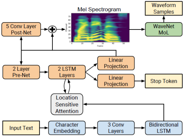
Flowtron learns an invertible function that maps a distribution over speech characteristics (mel spectrograms and text) to a latent z-space parametrized by a simple distribution (Gaussian). With this formalization, it can generate samples containing specific speech characteristics manifested in mel-spectrogram-space by finding and sampling the corresponding region in z-space. The output mel spectrograms are finally decoded into waveforms with WaveGlow, a universal decoder that generates high quality, natural-sounding speech.

The diagram describes the Flowtron network sequence including the Attention LSTM, Decoder LSTM, 2 Dense, Conv 1x1, and Affine Transform states. In z-space, the mel-spectrogram input is transformed in the affine coupling layer. — Figure 1. Flowtron network (not including the text encoder and the gate layer). Text and speaker embeddings are channel-wise concatenated. A 0-valued vector is concatenated with x in the time dimension.

Train with your own dataset

In addition to the public speech datasets such as LJSpeech (LJS), LibriTTS, M-AILABS, and so on, you can also train with your own dataset. We’ve heard common questions such as how to label your own dataset, how to remove background noise from the audio data, and so on. There are tools that can help you tag your dataset or remove background noise. To tag your dataset, you can try Amazon Mechanical Turk or use a semi-supervised approach for training a simple model to obtain labels from your data. For audio repair, iZotope RX delivers industry-standard audio repair tools including noise removal, dialogue isolate, and many other functions.

We recommend using 16-bit audio with a sampling rate of 22050 Hz. This bit-depth provides a good signal to noise ratio and the sampling rate provides a good inference-speed-to-audio-quality ratio because it covers most of the human voice frequency range (80Hz to 16kHz). Audio with higher bit-depth or sampling rate can be easily modified to match the audio setup just described. We do not recommend using a sampling rate lower than 22050 Hz.

To optimize training and memory consumption in large batches, we recommend using audio lengths of at most 10 seconds. It is possible to use longer audio files, but they might require you to decrease the batch size, which can increase model convergence time.

You can either train Flowtron from scratch if you have 10+ hours data for each speaker or fine-tune the pretrained models if you only have 15-30 minutes of data per speaker. The source code and pretrained models are shared in the NVIDIA/flowtron GitHub repo.

Training a Flowtron model from scratch is made faster by progressively adding steps of flow and using large amounts of data, compared to training multiple steps of flow at once and using small datasets. This progressive procedure and large amounts of data help the model learn attention quicker. Start by training Flowtron with a single step of flow (K=1) and progressively add steps of flow (K>1) when the K-th step of flow has learned to attend to the text, always training the full model. We evaluated models with one to six steps of flow and found that models with two steps of flow provide the best speech-quality-to-inference-time ratio.

We trained a Flowtron model (Flowtron-LSH) with two steps of flow for approximately 1000 epochs using the LJSpeech (LJS) dataset and two proprietary single speaker datasets, 20 hours from female speaker Sally and 10 hours from Helen.

Finally, the Flowtron-LSH model is fine tuned for 500 epochs on the train-clean-100 subset of LibriTTS, with 123 speakers. For LibriTTS, speakers with less than five minutes of data and files that are larger than 10 seconds were filtered out. Our Flowtron models were trained on uniformly sampled normalized text and ARPAbet encodings obtained from the CMU Pronouncing Dictionary. No data augmentation was performed.

Training Flowtron took less than 48 hours with the cuDNN-accelerated, PyTorch deep learning framework on a single NVIDIA DGX-1 with eight NVIDIA V100 GPUs. Based on our experimental results, Flowtron can achieve comparable MOS to Tacotron 2, as shown in Table.1. Moreover, Flowtron has the advantage of control over the speech variation and style transfer.

Source	Flows	MOS
Real	–	4.274 ± 0.1340
Flowtron	2	3.665 ± 0.1634
Tacotron2	–	3.521 ± 0.1721

Table 1. MOS evaluations with 95% confidence intervals for various sources.

For more information about the parameters to train Flowtron, see Flowtron: an Autoregressive Flow-based Generative Network for Text-to-Speech Synthesis.

Learning from our training experience, you can train Flowtron from scratch with your own dataset if you have 10+ hours of data per speaker, or you can fine-tune our pretrained models if you have models with 15-30 minutes data per speaker.

Customize variations and style transfer

The advantage of Flowtron over other state-of-the-art speech synthesis models is its capability for customization, without sacrificing speech quality. Flowtron samples show that you can control speech variation and apply unique styles to voices through style transfer, producing expressive speech without labeled data. These are barely achieved with other state-of-the-art models for speech synthesis, like Fastspeech or Tacotron 2.

As we mentioned earlier, Flowtron learns an invertible function that maps a distribution over speaking styles to a latent z-space parametrized by a standard Gaussian distribution. During inference, you can either sample from all speaking styles or sample from specific speaking styles.

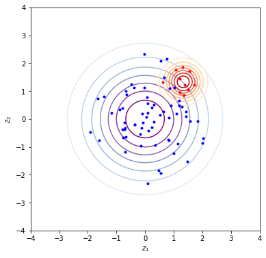
Figure 2 shows that sampling from all speaking styles is equivalent to sampling z-values from Flowtron’s entire z-space. This can be done by sampling z-values (blue dots) from a Gaussian with mean zero (blue circles) and adjusting the variance to control the spread of the Gaussian distribution. The hue of each circle is proportional to the chance of selecting a sample, which means that it is more likely to sample around the center than away from the center. Setting the variance to 0 corresponds to no variation in the generated speech and is equivalent to always using the central point. Increasing the variance corresponds to increasing the spread around the central point of the region in z-space being sampled, while maintaining samples closer to the center more likely than samples away from it. This can be used to control the amount of variation in the generated speech.

Sampling from specific speaking styles is equivalent to sampling from a specific region in Flowtron’s z-space, which is assumed to be another Gaussian distribution, that is associated with the speaking style. You can find the region in z-space that is associated with a specific speaking style by providing audio samples with the desired speaking style to Flowtron, obtaining z-values from them (red dots), and computing their centroid. Use this centroid as the mean of a Gaussian distribution (red circles) and adjust the variance one more time to adjust the span of the region in the z-space being sampled.

Standard Gaussian and Posterior diagram, with a Gaussian distribution in the upper left showing increased sampling. — *Figure 2. Illustration of a Gaussian distribution and Flowtron’s region in z-space associated with the style present in audio samples. Hue represents how often that region will be sampled.*

Sampling from all speaking styles

The simplest approach is to sample from a standard Gaussian distribution (the blue and purple circles in Figure 2) and adjust the amount of variation. The center point of the Gaussian distribution means no variation, and the variance can be increased by sampling from larger and larger circles.

Audio 1. No variation.

Audio 2. With variation.

Audio 3. Increased variation.

Flowtron can also perform interpolation in the latent space to achieve interpolation in the mel-spectrogram space. For example, linearly interpolating between two speakers Sally and Helen can create a speaker that combines the characteristics of both:

Audio 4. 100% Helen.

Audio 6. 66% Helen 33% Sally.

Audio 7. 33% Helen 66% Sally.

Audio 5. 100% Sally.

Instructions for sampling from all speaking styles

Initialize ${Z \sim \mathcal {N} (0, 1)}$ .
Sample ${z_{prior}}$ from ${Z}$ .
Perform inference with Flowtron using ${z_{prior}}$ and text.

Sampling from specific speaking styles

Another approach is to sample a posterior distribution containing speech characteristics found in observed samples and then interpolate between the prior standard Gaussian distribution and the posterior distribution to control the speaking style. In this way, Flowtron can make a monotonic speaker gradually sound more expressive.

Audio 8. Monotonic baseline.

Audio 9. Expressive rendition 1.

Audio 10. Expressive rendition 2.

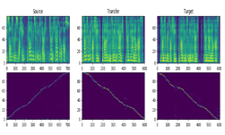
Flowtron can transfer acoustic characteristics from a style sample or speaker to a target speaker, so that the target speaker’s voice has the characteristics of the style reference. This is similar to style transfer in computer vision. For example, it can transfer the characteristics of a female speaker to a male speaker.

Audio 11. Source (male speaker).

Audio 12. Style (female speaker).

Audio 13. Target (male speaker with the characteristics of the female speaker).

In addition, Flowtron can transfer the style from data or speakers not seen in the training. Use style transfer to add different emotions to the baseline speaker by transferring that emotion from an unseen speaker in the training data or the unseen style of the seen speaker. For example, Flowtron can transfer the “surprised” style from speaker ID 03 of the RAVDESS emotional speech dataset to Sally. The result sounds drastically different from the monotonous baseline.

Audio 14. Baseline (Sally).

Audio 15. Style (surprised).

Audio 16. Target (Sally sounds surprised).

Instructions for sampling a specific speaking style

Collect evidence with mel and text with the specific style.
Create an empty list to store z values.
For each mel and text in evidence, do the following:
- Compute Flowtron’s z value: flowtron.forward(mel, text).
- Compute the average over time of the z value.
- Add the average over time to the z values list.
${\mu_ {posterior} \gets}$ Compute the mean over batch z values list.
# Initialize ${Z_{posterior} \sim \mathcal{N}(\mu_{posterior};0.25)}$
Sample ${z_{posterior}}$ from ${Z_{posterior}}$ .
Perform inference with Flowtron using ${z_{posterior}}$ and text.

Furthermore, you can sample from the Flowtron Gaussian mixture, which means that there are multiple distributions (imagine multiple collections of circles in Figure 2) corresponding to different speech characteristics. Modulate speech characteristics by translating one of the dimensions of an individual mixture component. For example, select a single component from the Gaussian mixture and translate a dimension associated with pitch. Although the samples have different pitch contours, they have similar duration.

Audio 19. μ – 4σ (e-flat).

Audio 18. μ – 2σ (c).

Audio 17. μ (a-flat).

Next steps

After reading this post and listening to the interesting samples, you can fork the NVIDIA/flowtron GitHub repo to get hands-on experience generating audio from text in real time and customize the audio at your preference. Start by using the pretrained models, which leads to faster convergence, especially if you only have a small dataset for fine tuning. There is also a COLAB notebook showing style transfer for you to play with.

A previous post, Generate Natural Sounding Speech from Text in Real Time, helps you provide English text to a model and have it generate an audio output file.